To kick off the blog section with a some developer coolness, I’ve decided to cover a small piece of code I invented a while ago. It is relatively tiny, but the process of getting there shows how much work goes into even the smallest building blocks of any software.
Introduction: Blend modes
As most of you likely know, image editing softwares like Photoshop have specific blending modes for their layers, which are formulas to describe how to mix one image into another. In fact, there’s a whole Wikipedia page dedicated to these formulas (https://en.wikipedia.org/wiki/Blend_modes).
One of the most commonly used blend modes is „Overlay“. You can use it to tint images or add some contrast. Photographers use it to give colors a certain „bite“ by overlaying a blurred version of the image onto the original image.
Here is the canonical formula:
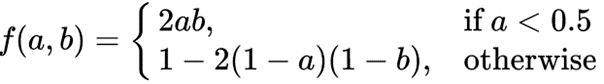
During some experiments with image tinting I obviously also experimented with Overlay, and found some peculiar stripe or rather discontinuity on the screen, which after quite some digging turned out to be caused by Overlay. Thinking that I maybe made a mistake implementing this (super simple) formula – wouldn’t be the first time – I fired up Photoshop and did some tests.
PROBLEM ANALYSIS
Indeed, if you overlay a horizontal gradient with a vertical gradient (which is a combo of all possible a and b together), there’s an ugly line across the image:

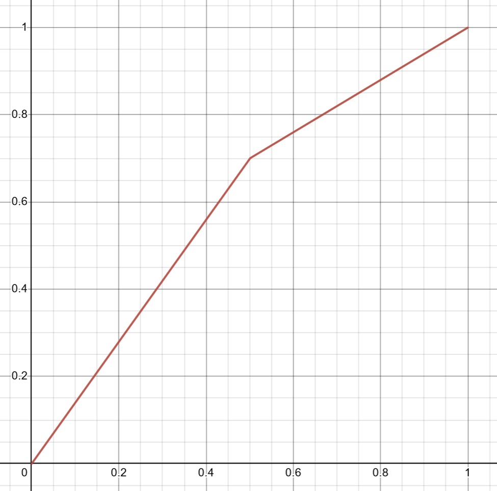
Evidently, the function is smooth everywhere, except at a = 0.5. A mathematician would say, its first derivative is discontinuous. The fact that it happens at a = 0.5 makes sense, as the curve is defined piecewise in respect to parameter a.
Plotting the curve with some static factor b shows this:
INTUITION OF THE SOLUTION
Now, in order to fix this, we need an alternative formula for the Overlay blend mode that behaves similarly, but is at least twice differentiable across this domain. Why twice? Well, you can’t calculate the derivative (or steepness) of a function at a jump. A curve with such a kink above has a jump in its first derivative, so you cannot differentiate it again at that location.
But let’s not get ahead of ourselves. First we need to find a way to reformulate the Overlay function that makes it easier or more intuitive to get to the source of the discontinuity. When modying a mathematical function, it always helps to strip away components. Since in this case, the curve goes from (0,0) to (1,1), stripping away f(x) = x from the curve, we are left with a triangle function:
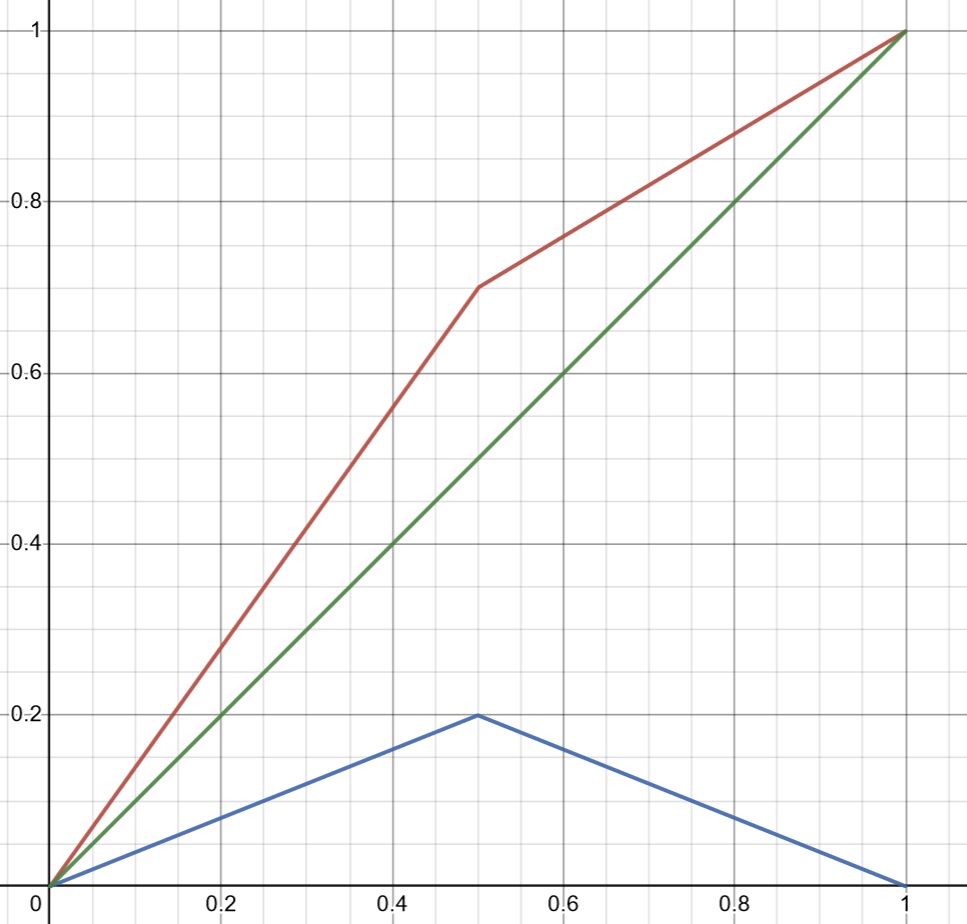
Now that’s easier to work with. By separating our function into two parts, only one of which has the kink in it, solving the problem now became simpler. y=x (green) is continuous so we only need to make the triangle function continous as well. And this is much easier than the sort of arbitrary function before.
FORMULATING THE SOLUTION
Assuming we can find a substitute for the triangle part, we still need to actually replace it in the Overlay function.
Therefore we need to reformulate the Overlay function in terms of a triangle function combined with something else so we can cleanly swap out the problematic part lateron. Let’s start with what we know:
- The height of the triangular part depends on the parameter b
- f(a, b=1) is maximally bent upwards, by a value of 0.5 compared to y=x
- f(a, b=0) is maximally bent downwards, by a value of -0.5 compared to y=x
- f(a, b=0.5) is a straight line, i.e. no triangular deformation up- or downwards
It is therefore reasonable to assume that the triangle is scaled by a factor of (b-0.5).
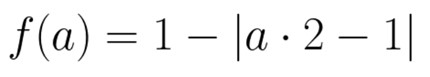
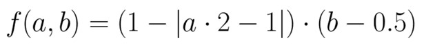
The formula for a triangle curve like the one above with height 1 is as follows:
Let’s incorporate the (b-0.5) scaling:
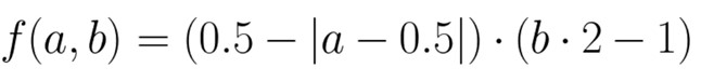
Now I found it easier to search for smooth triangle functions when their steepness is 1, which would result in a triangle with height 0.5, so this is the same formula but the left side describes a triangle with height 0.5. I merely multiplied the left side by 0.5 and the right side by 2 and simplified the formula.
What’s left is to add the second part of the overlay function again (the rising slope) which is just „a“, and we have the overlay function intuitively reformulated as a combo of a triangle function with something else:

To recap: We found the problem with the Overlay blend mode. We visually separated the function into the most minimal part that contains the problematic element vs the rest. We did this, so we can replace this part easier because a big function is more unwieldly. Then we did the same with the math formula for it, we found a new expression that does the same as the old blend mode formula, except now we also have this clean separation.
A really crappy smooth triangle is a simple parabola, which has the wanted properties of being twice differentiable – in fact all polynomials are infinitely differentiable, so if we can find a polynomial smooth triangle, we’re golden. Here’s x-x*x vs the triangle:
After trying it, it produced something really similar to Overlay, but it was too smooth for my tastes. Also, since the resulting curve must not exceed 1 or go below 0, our replacement must always be smaller or equal to the triangle itself!
At this point I immediately coded the solution because I know many different formulas but since this post is intended to illustrate the thought process when actually using high school math, pulling a formula out of a hat would probably seem unrewarding. So let’s try to derive it manually. It’s not complicated, I promise.
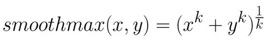
Now, the triangle itself is basically just the minimum of y=x and y=1-x. There is a plethora of smooth minimum formulas, some of which exploit the fact that in an arithmetic mean, raising each summand by some exponent k and raising the sum itself by 1/k makes it grow towards the maximum for rising k. And one can create a smooth minimum formula based off a smooth maximum formula.
Such a smooth maximum works like this:
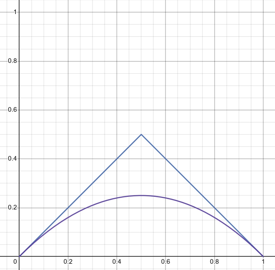
After turning it into a smooth minimum (inverting the inputs and inverting the output), it looks like this for various factors of k:
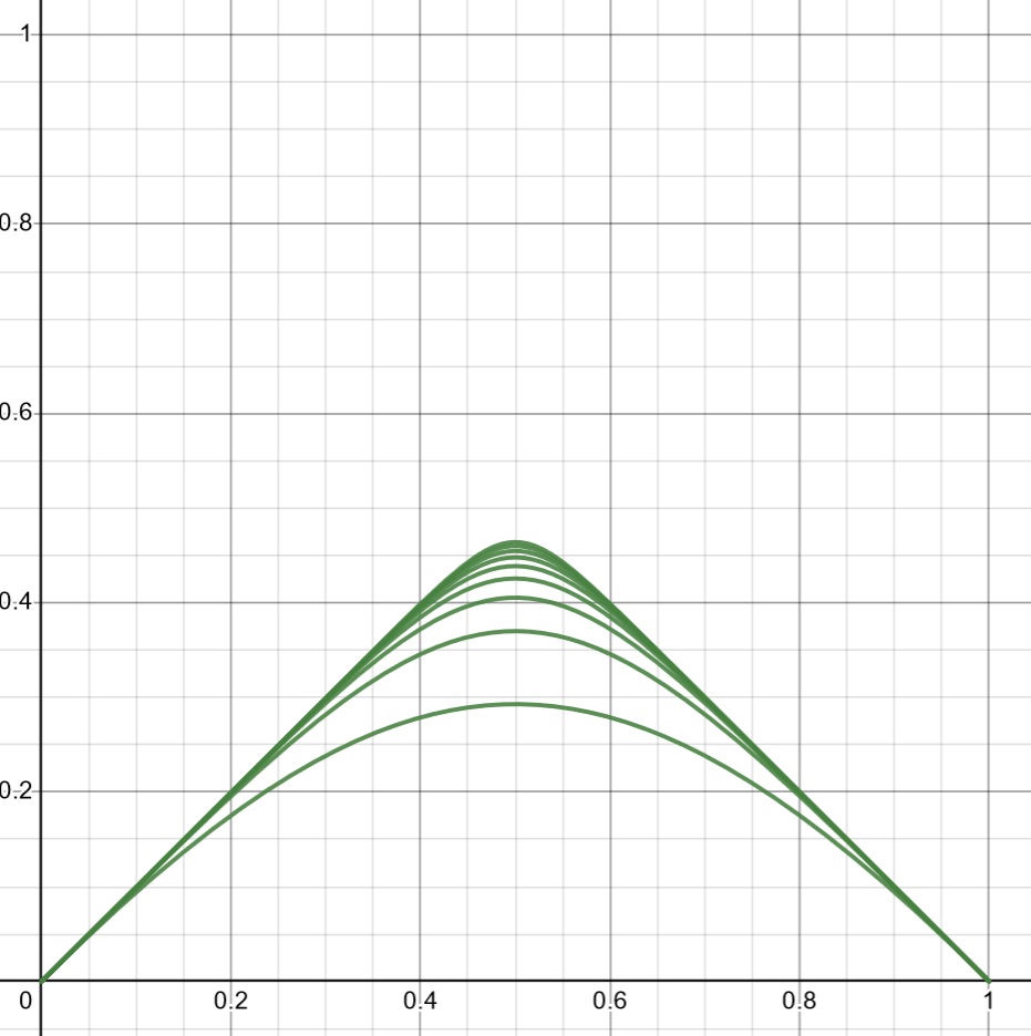
Perfect! Seems like we found our generic smooth triangle curve. It gets increasingly steeper with higher values for k, as for k towards infinity it approaches the true minimum, which is our original triangle. Fun fact: for k = 2 ( the lowest curve in the above diagram) we have our x – x*x, our original crappy triangle replacement.
Plugging it into the structure for our triangle curve based Overlay function, we get this:

That’s it! Let’s verify if it actually works, and indeed it does:

I’ve experimented which values produce the best results and 6-10 seems to be a good range. After all, we don’t want to alter the behavior of the curve at all, except at a very specific location. If we make it too sharp, that ugly line reappears, if we make it too smooth, it changes too much of the behavior across the entire value range.
As it turned out, Overlay was actually not a good pick for what I actually wanted to do, so it proved Knuth right yet again – premature optimization is the root of all evil. But it made for a fun math exercise and maybe you find this blog post inspiring.
Math really can be fun. Sometimes.